"yada, yada, yada" (Seinfeld and the Hebrew roots of knowledge)

Remember the Seinfeld episode in which George gets bent out of shape because his girlfriend omits some details to a story? She uses the phrase, "Yada, yada, yada" as if to gloss over mundane details with, "you know the rest." George, typical of his neurotic self, becomes obsessed and anxious that she is hiding something very significant from him by employing the yada, yada. The phrase has become common enough that most everyone will have heard or even used it interchangeably with, "Blah, blah, blah." Its etymology is elusive. However, if the phrase has any Jewish roots then it can plainly be linked to the idiom, "You know, you know, you know."

That is a long intro for a post that has nothing to do with Seinfeld and everything to do with the Hebrew verb for to know, "לדעת." Yada, in ancient Hebrew texts has a variety of meanings: to perceive, to understand, to demonstrate skill, to experience physical intimacy. Compare this to the modern sense of the word: assimilating all the data to uncover the object without bias from the subject. Also, compare this to the post modern sense of the word: a commodity exchanged between producers and consumers OR sense making for political expediency. Yada implies neither modern detachment nor post-modern game playing. The Hebrew sense of knowledge portrays a personal knower: from passion to perception to intellect to motor skill. For instance, the primitive metal worker and stone mason, Bezalel, was noted to have "knowledge" in various types of craftsmanship. Knowledge in this case would be a tacitly acquired skill for aesthetic construction. The ancient Hebrew king, David, employed the word "yada" in reference to how the night sky reveals the magnificence of God's glory. Knowledge in this case would be a visual perception of the object (the night sky) transfigured in relation to the subject's creator (see McGrath for this idea of the stars being transfigured into a sacramental mode).

Knowing a fact, knowing a person, knowing a skill, and knowing a feeling all require personal commitment on the part of the knower. The commitment is intellectual, relational, kinesthetic/tactile, and passionate. These functions of knowledge and the knower I hold to be properly basic in epistemology. Next post will focus on fleshing out these functions within my current field of study: epidemiology and yada, yada, yada.

solomon's judgement (or how the p-value is crazy like a fox)

Little Paul (that is me when I was a kid) listened to my father preach and teach many passages from the Bible. One impressionable passage Dad taught from was on King Solomon and his wise judgement when two women came to him claiming the other had stolen her child (I Kings 3:16-28). Being a busy potentate and one not all that interested in hearing the two mother's bicker back and forth all day, King Solomon suggested cutting the baby in half and letting them each take a half. Lo and behold, one woman saw this as a reasonable solution while the other was mortified at the suggestion. King Solomon's verdict: the true mother is the one whose immediate response is to protect the baby. The King was a wise judge; he elicited disparate responses from the two women and ruled based on a good hunch of how a true mother behaves. There is a very small probability that he awarded the baby to the non-biological mother (but, even with such an erroneous judgement he would have given the baby to a woman who wants to protect it and not cut it in half).

This case study in primitive law gets at the center of Fisher's p-value. Fisher, working largely in English agriculture, utilized probabilities (i.e.: p-values) to calculate how likely disparate responses would be among different crop samples under separate conditions for each sample. To do this he had to precede the statistical analysis with assumptions (or hunches) to draw conclusions (or judgments). For Fisher, the foundation was not math, but philosophical commitment to a body of prior learned knowledge that led to a priori presuppositions (beliefs held prior to investigation through which results are interpreted) and a posteriori inductions. Below I will touch lightly on the mathematical reasoning describing these commitments. These commitments are described by two terms: level of significance (a priori commitment) and p-values (a posteriori commitment).

Level of significance is a statistical term that reflects the probability of drawing a false conclusion. The closer the number is to zero, the lower the probability of drawing a false conclusion about groups being different; the closer the number is to one, the higher the probability of drawing a false conclusion. A 0.05 level of significance indicates that their is a 5% chance that a difference has been observed between two groups when in reality no difference exists (referred to as a type I error); a 0.10 level of significance means 10% chance of type I error, etc. This value can also be thought of as a false positive as demonstrated by the below 2 x 2 contingency table of hypothetical results versus hypothetical reality:

	Hypothetical Reality #1: Drug A = Drug B	Hypothetical Reality #2: Drug A ≠ Drug B
Hypothetical Result #1: Drug A ≠ Drug B	False Positive (This is termed “Level of Significance” and is synonymous with a Type I error...observing a difference when no difference truly exists.)	True Positive (This is termed “Power” because it is the power to find a true difference)
Hypothetical Result #2: Drug A = Drug B	True Negative (This is termed “Level of Confidence”)	False Negative (This is the definition of a Type II error...failing to find a difference when one truly exists)

Note that this is all hypothetical. The researcher sets this level of significance prior to the experiment; typically level of significance is set at 0.05. Then the researcher calculates a test statistic called a p-value. Any analysis that yields a p-value of less than 0.05 is considered significant and adds to the evidence that a true difference exists between groups. The p-value can only be obtained by assuming that the condition in box one (false positive) exists. That is, a p-value is calculated based on the assumption that in truth there is no difference between groups who have received different treatments. In other words, if two groups are treated with different diuretic drugs for high blood pressure, the researcher has a hunch that one drug is better than the other. To test the probability that his drug is superior to the other, he either must have access to the truth (which is not available in this kind of research design) or he must assume that there is no difference between the drugs and then test the observed difference against that assumption of no difference. So if he observes that his drug lowers blood pressure 10 points in the experimental groups and the other drug lowers blood pressure only 5 points in the control group, then the difference between the two drugs would be five (that is: 10-5 = 5). Assuming that there truly is no difference (hypothetical condition for box 1 in the above contingency table) he then subtracts the assumed difference (zero) from the observed difference (five) and divides this number by the standard error of the difference between both group means. Remember, standard error is a term used to reflect standard deviation of many experimental/control differences from the true mean if the experiment were repeated with random sampling from the population a large number of times. If the observed difference (5 in our example) is much larger than standard error (lets say standard error is 1 in our example), then the statistic will be large. The statistic can then be utilized to calculate a probability of observing the difference of 5 when the hypothetical reality of no difference is true. This is done by finding the test value on a normal bell curve and determining the area under the curve between that value and the left end of the curve. This area value is then the divided by the value of the entire area under the curve. The results in a probability of finding the difference between the two groups assuming that in truth there is no difference.

If any of you are still reading at this point, no doubt you are waiting for the point. Bottom line, the p-value, when smaller than the pre-set level of significance gives the researcher evidence that drug A truly is more effective than drug B. This is not a mathematical proof of the truth (only because the true situation is unknown), but rather mathematical support (or evidence) for one drug being better than the other. There may be Bayesian tricks (a la Neyman and Pearson) to guess at the true situation (termed prior probability) and then compare the results to this prior probability, however, even prior probability is based on a priori determination of values and so does not escape some personal judgement in the analysis. Fisher's p-value adds evidence one study at a time to slowly and over time produce a reliable body of knowledge. No one study creates definitive knowledge (diagnostic studies excluded). The best stewards of science recognize the valid role of personal judgement in arriving at true knowledge (see Michael Polanyi).

martial arts, global warming, and chance.

Scientific knowledge is produced piece meal through the slow process of research. One particular challenge in this process occurs when a researcher observes a difference between the experimental group and the control group. Did the difference arise because of chance or because of the experimental condition? Consider a child psychologist who is attempting to discern the most effective method for modifying explosive behaviors in children (say, ages 5 to 8). She designs a study in which the control group receives standard family counseling intervention while the treatment group receives standard family counseling plus Aikido martial arts training.

Suppose that the counseling + Aikido group exhibits a greater average reduction in explosive behaviors than the counseling alone group. What should the psychologist conclude? Was the difference really due to martial arts training? Or was there simply random variation between the two groups?

The observable world (a.k.a. the phenomenal or that which is accessible by our five senses) is characterized by variation. The world does have unifying undercurrents, however on the whole a vast multitude of divergent atomic structures abounds. In short, all things are not the same. There are alkali metals, alkaline earth metals, inert transition metals, transition metals and post-transition metals. There are tall people, short people, fat people, skinny people, brown skinned people, olive skinned people, red haired, brown eyed, toothy and toothless. Botanically, there are at least 40 different types of daffodils; each type of daffodil itself has a wide range of variable characteristics. This variation is what statisticians refer to when they use the terms "random error" or "random variation." On the other hand, variation due to some factor (e.g.: medication, exercise, psychotherapy, air pollution, etc) is referred to as explained variation. For example, consider an experiment which showed that lower carbon pollution levels curiously cause increased average temperatures in a simulated atmosphere.

Researchers want to know if this temperature variation is explained by reduced carbon pollution or by error (random variation). A high degree of variation in temperature recordings collected during the experiment may indicate that the average increase in temperature was a chance finding. In other words, if the variation in temperatures is great, then it may be that the researcher simply collected data during a time when temperatures were varying on the high end of the thermometer. Below I will show how the statisticians would answer the question, "Is the temperature rise due to the decreased carbon pollution or due to chance variation?"

When analyzing data sets from an experiment/study, researchers want to know if the observed change is a chance finding or a true reflection of how things really are. To do this they use a statistic called standard error (a quotient of standard deviation divided by the square root of the study sample size) to predict how variable the sample average would be if the experiment were repeated a large number of times. Essentially, the standard error statistic is used to calculate a range of values (termed "confidence interval") in which the researcher can be 95% confident that the true population average lies. Consider the atmospheric temperature study above. If the average temperature increased by 3.0 degrees Celsius, but the 95% confidence interval was -0.3 to 8.2 then it is entirely possible that no temperature change happened whatsoever (note that the value "0" is included in the range...indicating that the true average change in temperature may be 0 degrees Celsius). Such a scenario would indicate that the increase in temperature may truly be due to random variations or chance, not due to reduced carbon pollution.

Further testing can be done viz a viz Fisher's all powerful p-value to determine how insignificant the temperature rise truly is. In fact, selecting levels of significance and calculation of p-values will be the topic of next post. From there I will switch out of statistics mode and into philosophy mode.

descriptive stats revisited

Last post I attempted a brief and somewhat unclear introduction to descriptive statistics. So by way of review I will summarize last post with a graph to help depict things. The three most basic ways of describing a data set are its average, spread and shape. These three concepts are very important as performing statistical analysis depends on these three descriptions of the data being "normal." The average of the data set represents where the majority of the data lie. A normally distributed set of data (referred to as a bell curve when plotted) will have an obvious mean at the peak of that curve. See how on the normal curve below, the line representing the mean divides the curve into two symmetric halves.

The spread of the data indicates to what degree all the data points vary away from the average. Standard deviation is a number that indicates the average distance of all data points from the average. Higher standard deviations indicate that the range of data spread further on either side of the average. See the lines on either side of the central average line on the graph below? The first line on either side of the average line indicates a point that is 1 standard deviation from the mean. The next line indicates a point that is 2 standard deviations away from the mean. Particular to the normal bell curve is the reality that 67% of all data will be only one standard deviation from the mean and 95% of the data only 2 standard deviations away from the mean.

The shape indicates whether the bell curve has a long tail to the left [negative skew], long tail to the right [positive skew], tall curve [leptokurtic], flat cruve platykurtic). Any distortion of the bell curve impacts statistical calculations as basic statistics assume a normal bell curve. See below for depictions of skewed data.

Next post I will answer the following question: how do we know if the difference between two groups or two measurements is due to chance or due to skill or treatment effect?

redlegs and descriptive stats

Honestly, my appreciation of baseball is pathetic. That is a veritable reality (as those acquainted with me can attest). However, as a youth I followed Redlegs baseball compulsively. Sunday mornings were great because the Cincinnati Enquirer would have an expanded sports section with all the breakdown of player and team stats (this was before the dawn of ESPN.com/mlb/statistics....in a former age when all fans waited with baited breath for our information to arrive through the paper delivery man). Batting averages, ERA's, standings, etc. Typical of my analytic approach to things, I would perform my own calculations to see how many hits Hal Morris would need to break .400 over the next 50 at bats. Much has changed since my youth, but I still gain a good deal of satisfaction in performing calculations. For those who might find such a thought foreign or even perverse, I will frame this post on summary statistics around baseball. Perhaps no one will even notice that math is being conducted.

Data collection is the process of compiling bits of information (e.g.: number of hits, innings pitched) in an organized system (I personally prefer Excel for its ubiquitous use). Without doing at least some basic calculations the data are not very meaningful. Summary statistics are employed to describe several qualities of the data: location, spread, and shape. Location captures where the majority of the data lie (e.g.: the team batting average represents a central number around which most of the players on a baseball team are averaging). Spread captures how widely the data varies (e.g.: once the location is known we want to know how big the difference is between the worst batting average and the best batting average). Shape captures how closely a graph of the data resembles a bell shaped curve (e.g.: if the batting average is relatively high compared to the spread of individual batting averages then the shape will be abnormally tall and departs from a normal bell curve). In statistical jargon these three qualities are referred to as: mean, variance and skewness/kurtosis. (WARNING: those who experience anxiety when exposed to mathematical formulas should skip over the next paragraph...you won't miss much).

Mean is the sum of the data divided by the number of data points and is denote by the upper case "Y" with a line over it in the equation:

.

Variance is the square of each data points distance from the mean, all summed and divided by total number of data points minus 1. The square root of variance can then be taken to reflect the average distance that data points vary from the mean

.

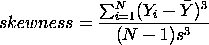
Skewness is obtained by the cubed value of (the mean subtracted from each data point), summed for all data points and then divided by the product of (total number of data points minus 1) and (the cube of standard deviation). When this number is significantly positive then the data is not normally shaped and is lopsided to the right; when this number is negative then the data is lopsided to the left. Kurtosis is obtained similarly to skewness only the numerator is taken to the 4th power and standard deviation in the denominator is taken to the 4th power . 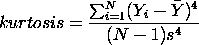A significantly negative kurtosis number indicates a flat curve and a positive kurtosis number indicates a tall, lanky curve.

Why are descriptive statistics important? There is a phenomenon out there in the sports world known as fanaticism. A true baseball fanatic will go to extreme lengths to stand by her team. It is even conceivable that during pleasant interchange over brews she may overstate or even understate the skill level of her team. In the world of statistics we call this bias. Descriptive statistics help us to reduce the influence of bias and see things more like they really are. No matter how devoted I am to the Redlegs offense, if I compare a variety of reliable offensive indicators to the same indicators for the Cardinals, I will find out the truth of how well they compare. If we compare the two teams and find that the Redlegs have better numbers and that the difference between the two teams is not due to chance, then I may not only brag as a fanatic but as a man who knows the statistical truth ("statistical truth," is that an oxymoron?).

So that raises a question, how would I know if the better Redlegs numbers were due to chance or skill? Tune in to next post for a breathtaking answer.

ents

Last post I mentioned that this post would be a technical one on statistics. However, after studying further on the subject of statistics I quickly realized that I am not qualified to author a technical post on the matter. Instead I will here offer a post that works to hold together statistics and scientific epistemology. Think of scientific epistemology being somewhat like Tolkien's tree Ents that he depicted as gathering around in a counsel to decide on a course of action. They refuse to be rushed in their decision making by the immediacy of danger: rather they thoroughly work the problem over to ensure that their decision places them on the side of good. Likewise with scientific epistemology, establishment of true knowledge occurs slowly and without any deference to the urgent need of human beings. So here ensues an elaboration of Ent-like knowledge building interspersed with pictures of past heroes of statistics (everybody should choose at least one statistical hero...such a thing ought to be as ubiquitous as having a NASCAR driver to root for).

I believe that natural human knowledge is capable of more than a mere approximation of reality. I believe that natural human knowledge can achieve a one-to-one relationship with reality; that is to say that theories of reality (i.e.: how things are) can represent specified slices of reality with perfect accuracy (e.g.: Copernicus and heliocentrism; Newton and gravitational forces, etc.). However, I also believe that the vast majority of natural knowledge produced in a given calendar year is specious at worst (i.e.: false knowledge) and an approximation of reality at best (i.e.: analogous knowledge). Here I refer not to the sort of assertions that pass off as knowledge among the popular pundits, but rather I am referring to critically tested, peer-reviewed scientific knowledge. It is this high level of knowledge that ranges from false to analogous. To characterize this range of knowledge quality I have generated a list of four (4) descriptors beginning with the most basic and contingent sort of knowledge progressing up to true knowledge or "fact" (as science would have us call it).

Ronald Fisher: what's not to like about this statistician? The very incarnation of an Ent.

Possible. Definition: that can be; capable of existing. For example an oval circle is quite possible; an oblong circle is quite possible. However, a square circle could never be a circle (i.e.: essentialistically impossible). An MRI machine that produces only rare cheese could never be an MRI machine (i.e.: nominalistically impossible). Certain things are impossible. Importantly, though, many possible things are not true. For instance, although it is possible for a live cow to go over the moon, if I claim to know that a live cow actually went over the moon last night this would be a false knowledge claim. Although it is possible for the sun to rise in the West and set in the East, this is not the truth of what happens on planet Earth. That which is conceivably possible is not necessarily existentially so. This being held true, there are three possible descriptions of possibilities and existence: existent possibility, nonexistent possibility, nonexistent impossibility. There is no such thing as an existent impossibility.

Karl Pearson: note with what alacrity he wields his pen in noble service of statistics.

Probable. Definition: likely to occur or to be so; that can reasonably be expected or believed on the basis of the available evidence, though not proved or certain. For example, a 2002 study published in Spine journal deduced a clinical prediction rule to identify which patients with low back pain are most likely to be successfully treated with spinal manipulation. The study deduced these 5 parts for a prediction rule: 1) pain onset less than 16 days prior to treatment; 2) no symptoms distal to the knee; 3) Fear Avoidance Behavior Questionnaire score less than or equal to 19; 4) one or more hypomobile segments in the lumbar spine; 5) at least one hip with more than 35 degrees of internal rotation motion. A patient must exhibit at least 4 of the above 5 traits to be considered positive on the rule. A subsequent randomized controlled trial published in 2004 compared patients who satisfy this rule with those who do not. They found that patients positive on the rule and receiving spinal manipulation have an adjusted odds ratio for successful treatment of 60.8 when compared to those negative on the rule and receiving exercise. That is to say, a person who satisfies the prediction rule and is treated with spinal manipulation is 60.8 times more likely to have a successful outcome than someone negative on the rule and receiving exercise. Although adjusted odds ratios are not exactly probabilities, they approximate mathematical probabilities closely when baseline risks are low. Consequently we can say that a person with low back pain who satisfies the prediction rule is very likely to gain significant function after only 2 treatments of spinal manipulation and this functional gain is likely to last for 6 months. But, this is a probability. This means that a small number of people who are positive on the rule and receive spinal manipulation will feel no improvement or worsening symptoms after treatment. So this is a practical example of probabilistic knowledge. The above studies did not elucidate fact, they elucidated pragmatic probabilities to help clinicians, insurance companies and patients make a decision about treatment options.

Valid. Definition: sound; well grounded on principles or evidence; able to withstand criticism or objection, as an argument. The move from probable knowledge up to valid knowledge is like passing over the Natural Light beer for Kentucky Bourbon Barrel Ale. Like declining the Hostess Snack Cake to save room for Graeter's ice cream. Like operating on the spine with a high precision Medtronic drill instead of a high speed DeWalt house drill. Valid knowledge within medical diagnostics is produced when a new test for diagnosis is measured against a gold standard. Assessing the new test (lets say for detecting prostate cancer) against the gold standard can result in four possible outcomes: true positive, false positive, true negative, and false negative. The box below illustrates this well:

	Gold Standard Negative (no prostate cancer present)	Gold Standard Positive (prostate cancer present)
New Test Positive	False Positive (invalid test result)	True Positive (valid test result)
New Test Negative	True Negative (valid test result)	False Negative (invalid test result)

A variety of statistics are available to describe these results, however I will spare the reader details of these at this time. Let the reader note, though, that validity does not measure probability of departure from truth but rather it measures reality of departure from truth. In this way validity is not a guess at the truth but a true measure of the truth. The greatest mistake in popular conceptions of research occurs when studies analyzed by probabilistic statistics (i.e.: p-values and confidence intervals) are interpreted as if they utilize validity statistics (i.e.: likelihood ratios). In this manner, many studies are presented as valid when they ought truthfully be presented as some grade (e.g.: low, moderate, high grade) of probabilistic evidence for or against a hypothesis.

Thomas Bayes: the right Reverend had a penchant for more than divine truth.

Veritable. Definition: true; real; actual. I am taking the name of this descriptor from the Latin word veritas: truth. How does the descriptor "veritable" differ from the descriptor "valid"? Knowledge that is veritable is perfectly true (1-for-1 correspondence with reality or logic) whereas knowledge that is described by validity is expressed as a degree of departure from truth. Given the above diagnostic example: the new prostate cancer test would be characterized as being valid if it deviates from the gold standard to only a small degree and invalid if it deviates from the gold standard to a large degree. However, the gold standard test is veritable: a container of 100% true knowledge, finding prostate cancer whenever it exists and ruling out prostate cancer whenever it does not exist. Veritable knowledge is not simply produced by a mathematical formula, but is rather arrived at through years of practice, research (statistically analyzed), critical review (e.g.: statistical assessment, construct assessment, etc.), technical reformulation, and even large scale disciplinary enactment (i.e.: use within the guild at large).

Jerzy Neyman: a fierce opponent to Fisher; his calculations were as killer as his Hitler-ish look.

One final cautionary note is due here. Having moved through this post, and engaged with the proposed hierarchical categories of knowledge (low quality "possibility" knowledge up to highest quality "veritable" knowledge) the reader might be tempted to scorn knowledge that is beneath "veritable" in my hierarchical scheme. The purpose of these hierarchies is not to cast aspersion upon "inferior" knowledge, but rather to appropriately characterize the levels of knowledge and their relation to truth. This has very pragmatic implications. Possible knowledge should be utilized with extreme caution and proposed lightly with a ready willingness to believe alternative possibilities; probable knowledge should be utilized discriminantly and defended publicly with openness to evidence to the contrary; valid knowledge should be ubiquitously employed and publicly defended with great vigor and energy; veritable knowledge should be published and re-published with regular frequency as well as being proclaimed with certainty to winsomely disabuse falsehoods consistently where falsehoods appear.

Next post will be devoted to a description of basic statistics and some of their mathematical formulations.

monochrome

Two and one half years have ticked off the mantle top clock since the last post on this blog. Even more embarrassing is a swift look at the goals mentioned in that last post: publishing a case study in the national physical therapy journal (that didn't happen), become a researcher (not much traction on that over 2.5 years), becoming a voice that shapes physical therapy knowledge (I haven't even started talking yet). Alas and alack, my life was actually interesting over the last couple years: job changes, selling/buying a house, first born daughter arrived on the scene, theological growth, starting graduate classes again. No time for the monochrome world of research. I had some life to live. Life is settling down a little now. Hopefully a little more tranquility will invade my work life over the coming months and then I can really begin in earnest tackling scientific epistemology viz a vi statistics and clinical research.

Interestingly enough, my introduction to biostatistics course this summer is a refreshing reminder that learning is fun. My instructors Drs. Shukla and Dwivedi are doing a superb job of instructing the class at a philosophical level. They are engaging questions of statistical certainty within the constraints of probabilistic mathematics (a world they refer to as fuzzy or gray) counterbalancing the clinical drive for a definite answer for ailing patients. The most unique concept I have learned to date is this: hypothesis testing (i.e.: level of significance and p-value) does not result in a mathematical acceptance or rejection of the hypothesis. Rather, hypothesis testing adds or removes weight to an a priori belief that the hypothesis is true. In this manner, statistics are legal procedures. The test statistic is the prosecuting trial attorney arguing the state's case in front of the judge and jury. The data is considered insignificant unless otherwise proven beyond reasonable doubt by the test statistic.

Next post will be a technical one exploring some aspect of statistics and how they relate to contemporary medical knowledge.